Gaussian distribution

Why is the Gaussian distribution often used instead of a simpler uniform distribution in lattice-based cryptography?

In many lattice-based cryptographic schemes, such as Learning With Errors (LWE) and Ring-LWE, random noise is added to make certain problems difficult to solve (e.g., distinguishing between an exact solution and one with small error). Gaussian distributions are well-suited for modeling this noise because most of the noise is close to the mean, but there’s a small probability of larger deviations which makes it challenging for attackers to predict and remove the noise.

But there’s another reason the Gaussian distribution is used. In lattice-based cryptography, you often don’t know the lattice is because it’s part of someone’s secret key. For example, for the private key, we use a good basis that represents the same lattice as the bad basis. The bad basis describes the lattice well enough to make hiding the message a hard problem on the lattice.

How can you sample error vectors uniformly if you don’t know the lattice?

Let’s consider a one dimensional lattice, $\mathbb{Z}$, and pretend we don’t know it (it might be $2\mathbb{Z}$ or $\frac{3}{4}\mathbb{Z}$ or whatever).

If you simply take a uniform interval, say $[\frac{1}{4}, \frac{3}{4}]$, the differences (error vectors) between the uniformly random sampled values and the lattice vectors won’t be uniformly distributed. If you take a very large interval, the error vectors will be closer to the uniform distribution, but this creates issues in the security proofs.

However, the Gaussian distribution has a very nice property—it approximates a uniform distribution modulo a lattice exponentially well, regardless of the lattice. This means that if we take the differences (error vectors) between the samples from the Gaussian distribution and the lattice vectors (whatever they may be), these differences will be uniformly sampled.

For some intuition, let’s consider the following exmample. Suppose we have the lattice $\mathbb{Z}$. The probability of sampling, for example, the value $0.7$ is very similar to that of any other value. Now, let’s say that the points $A$ and $B$ in the image correspond to $A = -0.3$ and $B = 0.7$. In fact, both values present $0.7$ because we consider the difference from the closest lattice vector that is smaller than the sampled value (see fractional part (opens new window)).

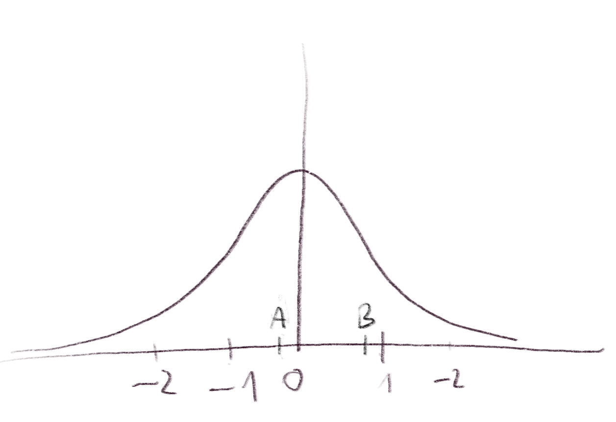
The probability of obtaining the error vector $0.7$ is almost the same as the probability, for example, of obtaining $0.2$. Suposse we sampled $C = -0.8$ and $D = 0.2$. Both correspond to the error vector $0.2$. Intuitively, we can see that the probability obtaining $0.2$ is the same as the probability of obtaining $0.7$ because $D$ is sampled with higher probability than $B$, but on the other hand, $C$ is sampled with lower probability than $A$.

The larger the standard deviation, the closer the distribution of the error vectors becomes to the uniform distribution.

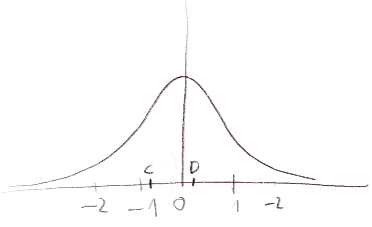
The same holds true if we use a different lattice, such as $2 \mathbb{Z}$.

The most compact lattice-based signature schemes require the Gaussian distribution, but it is important to note that making it secure against side-channel attacks is challenging, and its implementation is highly non-trivial.